import os
import tempfile

import numpy as np
import plotly.graph_objects as go

import nefes
from nefes.thermo import SpeciesDatabase, Thermo, EQ_FROZEN, EQ_KERNEL
from nefes.chem import resolve_composition, enthalpy_mass, equivalence_ratio_mixture
from nefes.elements import catalog as cat
from nefes.plotting import use_nefes_theme, COLORWAY

# Use the bundled theme instead of plotly's default.
use_nefes_theme()

R_AIR, GAMMA = 287.0, 1.4
CP = GAMMA * R_AIR / (GAMMA - 1.0)Reacting-flow fundamentals
The building blocks behind the combustor examples: fuel injection, a heat-release flame, and the frozen and equilibrium gas states.
Source notebook: examples/combustion/reacting_flame.ipynb. This page is executed from it at build time.
The building blocks behind the combustor examples:
nefes.thermoHP equilibrium: the adiabatic flame temperature vs. equivalence ratio, straight from the NASA thermochemical data (no network);- the perfect-gas heat-release flame: a prescribed power
Qdotraising the total temperature; - the reacting equilibrium flame: frozen unburnt reactants in, equilibrium products out, the flame temperature emerging from the solve.
1. Adiabatic flame temperature vs. equivalence ratio (thermochemistry only)
Standalone chemical equilibrium: build a small H2/air library, then solve HP equilibrium of the reactant elements at the reactant enthalpy.
lib = SpeciesDatabase().select(["H2", "O2", "N2", "H2O", "OH", "H", "O", "HO2", "NO"])
gas = Thermo(lib)

AIR = {"O2": 0.21, "N2": 0.79}  # dry air (mole)


def h2_air(phi):
    """H2/air mixture at equivalence ratio phi (mole), via the Nefes mixture helper.

    ``equivalence_ratio_mixture`` fixes the stoichiometric H2/air ratio from the
    elemental oxygen balance: no hand-tuned 0.5 O2 / 3.76 N2 bookkeeping.
    """
    return equivalence_ratio_mixture({"H2": 1.0}, AIR, phi, species_set=lib)


phis = np.linspace(0.4, 1.6, 13)
Tad = []
for phi in phis:
    Y, Z = resolve_composition(lib, h2_air(phi), basis="mole")
    h = enthalpy_mass(lib, Y, 300.0)
    eq = gas.equilibrate_HP(Z, h, 101325.0, T_guess=2000.0)
    Tad.append(eq.T)

fig = go.Figure()
fig.add_scatter(x=phis, y=Tad, mode="lines+markers", line_color=COLORWAY[4])
fig.update_layout(
    title="H₂/air adiabatic flame temperature (HP equilibrium)",
    xaxis_title="equivalence ratio  φ",
    yaxis_title="adiabatic flame T  [K]",
    showlegend=False,
    height=440,
)
fig.show()
print(f"peak Tad = {max(Tad):.1f} K near phi = {phis[int(np.argmax(Tad))]:.2f}")
peak Tad = 2391.7 K near phi = 1.102. Perfect-gas heat-release flame
A 2-port flame that adds a prescribed power Qdot [W]; the total temperature rises by Qdot / (mdot * cp), mass and the constant-area momentum flux are conserved (a Rayleigh static-pressure drop appears).
mdot, Tt, Qdot, A = 10.0, 300.0, 2.0e6, 0.05
net = nefes.Network(
    nefes.perfect_gas(R_AIR, GAMMA),
    nodes=[cat.mass_flow_inlet(mdot, Tt), cat.heat_release_flame(Qdot), cat.pressure_outlet(1.0e5)],
    edges=[(0, 1, A), (1, 2, A)],
)
sol = net.solve()
assert sol.converged, (sol.residual_norm, sol.print_residuals())
unburnt, burnt = sol.edge(0), sol.edge(1)
print("converged:", sol.converged)
print(f"  Tt in/out : {unburnt['h_t'] / CP:.1f} -> {burnt['h_t'] / CP:.1f} K  (predicted +{Qdot / (mdot * CP):.1f} K)")
print(f"  static T  : {unburnt['T']:.1f} -> {burnt['T']:.1f} K")
print(f"  static p  : {unburnt['p'] / 1e3:.2f} -> {burnt['p'] / 1e3:.2f} kPa (Rayleigh drop)")
imp = [sol.edge(e)["rho"] * sol.edge(e)["u"] ** 2 + sol.edge(e)["p"] for e in (0, 1)]
print(f"  momentum flux rho*u^2 + p conserved: {imp[0]:.1f} vs {imp[1]:.1f} Pa")
converged: True
Tt in/out : 300.0 -> 499.1 K (predicted +199.1 K)
static T : 291.4 -> 463.8 K
static p : 126.89 -> 100.00 kPa (Rayleigh drop)
momentum flux rho*u^2 + p conserved: 153246.8 vs 153246.8 Pa3. Reacting equilibrium flame (single premixed stream)
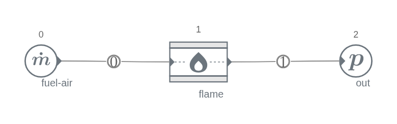
Frozen H2/air approach -> equilibrium products. ‘Ignition’ is the per-edge closure switch: the approach edge is EQ_FROZEN, the product edge EQ_KERNEL. The premixed H2/air is a single feed stream (one transported mixture fraction, discovered from the inlet composition at build time), and net.solve() seeds itself by propagating the feed through the network: no hand-built guess.
phi = 1.0
Y, Z = resolve_composition(lib, h2_air(phi), basis="mole")
h_react = enthalpy_mass(lib, Y, 300.0)
mdot, p, A = 1.0, 101325.0, 0.05

net = nefes.Network(
    nefes.equilibrium(lib),
    nodes=[
        cat.mass_flow_inlet(mdot, 300.0, composition=h2_air(phi), name="fuel-air"),
        cat.equilibrium_flame(name="flame"),
        cat.pressure_outlet(p, Tt_backflow=300.0, composition=h2_air(phi), name="out"),
    ],
    edges=[(0, 1, A), (1, 2, A)],
    edge_models=[EQ_FROZEN, EQ_KERNEL],
)
sol = net.solve()
assert sol.converged, (sol.residual_norm, sol.print_residuals())
unburnt, burnt = sol.edge(0), sol.edge(1)
ref = gas.equilibrate_HP(Z, h_react, burnt["p"], T_guess=2000.0)
print("converged:", sol.converged)
print(f"  unburnt T : {unburnt['T']:.1f} K     burnt T : {burnt['T']:.1f} K")
print(f"  standalone HP-equilibrium reference : {ref.T:.1f} K")
print(f"  density dilatation rho_u/rho_b = {unburnt['rho'] / burnt['rho']:.2f}")
converged: True
unburnt T : 299.8 K burnt T : 2374.3 K
standalone HP-equilibrium reference : 2379.0 K
density dilatation rho_u/rho_b = 7.01Equivalence-ratio sweep through the network
The network flame temperature tracks the standalone adiabatic flame temperature.
phis2 = np.linspace(0.5, 1.4, 10)
Tnet, Tref = [], []
for phi in phis2:
    Y, Z = resolve_composition(lib, h2_air(phi), basis="mole")
    h_react = enthalpy_mass(lib, Y, 300.0)
    s = nefes.Network(
        nefes.equilibrium(lib),
        nodes=[
            cat.mass_flow_inlet(1.0, 300.0, composition=h2_air(phi)),
            cat.equilibrium_flame(),
            cat.pressure_outlet(101325.0, Tt_backflow=300.0, composition=h2_air(phi)),
        ],
        edges=[(0, 1, 0.05), (1, 2, 0.05)],
        edge_models=[EQ_FROZEN, EQ_KERNEL],
    ).solve()
    assert s.converged, (s.residual_norm, s.print_residuals())
    Tnet.append(s.edge(1)["T"])
    Tref.append(gas.equilibrate_HP(Z, h_react, s.edge(1)["p"], T_guess=2000.0).T)

fig = go.Figure()
fig.add_scatter(
    x=phis2, y=Tref, mode="lines", name="standalone HP equilibrium", line=dict(color=COLORWAY[0], width=4), opacity=0.5
)
fig.add_scatter(x=phis2, y=Tnet, mode="markers", name="network flame", marker=dict(color=COLORWAY[4], size=9))
fig.update_layout(
    title="Network flame vs. standalone equilibrium",
    xaxis_title="equivalence ratio  φ",
    yaxis_title="burnt T  [K]",
    height=440,
)
fig.show()
Export for Nemo
The reacting network net and its converged mean flow sol are already in scope. Save either to a UI-readable YAML: sol.to_yaml(path) embeds the mean-flow result fields, net.to_yaml(path) writes the topology only: then open the file in Nemo.
_out = os.path.join(tempfile.mkdtemp(), "reacting_flame.yaml")
sol.to_yaml(_out)  # embeds the mean-flow results; use net.to_yaml(_out) for topology only
print("saved case:", _out)
saved case: /tmp/tmp6qqom2eu/reacting_flame.yaml