Helmholtz resonator

Build a Helmholtz resonator and see how the storage block M enters the acoustic operator A(omega).

Source notebook: examples/acoustics/helmholtz_resonator.ipynb. This page is executed from it at build time.

The acoustic operator is \mathbf A(\omega)=\mathbf J_{\mathrm{alg}}+i\omega\mathbf M+\mathbf P(\omega)+\mathbf S(\omega). This notebook demonstrates the storage block \mathbf M, newly populated by a single new element: the cavity.

A cavity(V) is a wall to the mean flow (\dot m=0) and a compliance to acoustics: its enclosed gas compresses isentropically, storing energy with lumped compliance

C=\frac{V}{\overline\rho\,\overline c^{\,2}},

which populates \mathbf M with the single coefficient V/\overline c^{\,2} on the cavity’s mass row.

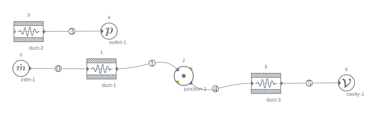
The Helmholtz resonator itself is not a new element: it is composed from the existing primitives: a junction (the tee), a short duct (the neck inertance L_a=\overline\rho\,\ell/A_n), and the new cavity (the compliance C). The resonance

\overline f_0=\frac{\overline c}{2\pi}\sqrt{\frac{A_n}{V\,\ell}}\qquad\Bigl(\omega_0=\tfrac1{\sqrt{L_aC}}\Bigr)

then emerges from those parts wired together: it is coded into no single element.

import numpy as np
import plotly.graph_objects as go

import nefes
from nefes.elements import catalog as cat
from nefes.plotting import use_nefes_theme, COLORWAY

use_nefes_theme()

#  --- calorically perfect air at rest ---
GAMMA, R = 1.4, 287.0
GAS = nefes.perfect_gas(R, GAMMA)
P0, T0 = 101325.0, 300.0
C0 = np.sqrt(GAMMA * R * T0)  # sound speed [m/s]
RHO0 = P0 / (R * T0)  # density [kg/m^3]

#  --- resonator geometry ---
S_MAIN = 3.0e-3  # main-duct area [m^2]
A_NECK = 5.0e-4  # neck area [m^2]
L_NECK = 0.03  # neck length [m]
V_CAV = 2.0e-3  # cavity volume [m^3]
L_MAIN = 0.08  # main-duct half-length each side (compact) [m]


def helmholtz_f0(c, An, V, l):
    """Analytic Helmholtz frequency f0 = c*sqrt(An/(V*l)) / 2pi [Hz]."""
    return c * np.sqrt(An / (V * l)) / (2.0 * np.pi)


print(f"c0   = {C0:.1f} m/s,  rho0 = {RHO0:.4f} kg/m^3")
print(f"f0   = {helmholtz_f0(C0, A_NECK, V_CAV, L_NECK):.1f} Hz   (analytic Helmholtz frequency)")

c0   = 347.2 m/s,  rho0 = 1.1768 kg/m^3
f0   = 159.5 Hz   (analytic Helmholtz frequency)

Part 1: the `cavity` is a compliance

Build the simplest storage network: a driven port, a neck duct, and the cavity dead-end (inlet → neck duct → cavity). The cavity blocks the mean flow (\dot m=0, exactly a wall), and its finite volume contributes one entry to \mathbf M: the compliance V/\overline c^{\,2} on the cavity’s mass row.

def neck_cavity(volume, neck_len, neck_area):
    net = nefes.Network(GAS)
    inlet = net.add(cat.total_pressure_inlet(P0, T0))  # quiescent driver, pins the pressure level
    neck = net.add(cat.duct(neck_len))
    cav = net.add(cat.cavity(volume))
    net.connect(inlet, neck, neck_area)
    e_cav = net.connect(neck, cav, neck_area)
    sol = net.solve()
    assert sol.converged
    return sol, cav, e_cav


sol1, cav_node, e_cav = neck_cavity(V_CAV, L_NECK, A_NECK)

# mean flow: the cavity is a wall -> mdot = 0 everywhere
print(f"max |mdot| in the network = {np.max(np.abs(sol1.field('mdot'))):.2e} kg/s   (cavity blocks the mean flow)")

# the cavity's finite volume is a compliance C = V / c^2: the single coefficient it stamps into
# the storage block M on its own mass row.
c_cav = sol1.edge(e_cav)["c"]
print(f"\ncavity compliance  C = V / c^2 = {V_CAV / c_cav**2:.6e}")

max |mdot| in the network = 0.00e+00 kg/s   (cavity blocks the mean flow)

cavity compliance  C = V / c^2 = 1.659200e-08

Result. The mean flow is quiescent (\dot m\to0: the cavity is a wall), and its finite volume contributes exactly one coefficient, C=V/\overline c^{\,2}, on the cavity’s mass row. That single entry is the compliance: combined with the neck duct’s inertance it produces the resonance demonstrated next.

Part 2: the Helmholtz resonator, composed from primitives

Now place the neck + cavity as a side branch on a main duct, off a junction:

At \overline f_0 the series neck-inertance / cavity-compliance branch impedance Z_b=i(\omega L_a-1/\omega C) passes through zero, shorting the junction pressure: a sharp transmission-loss peak. We compare the Nefes network against the analytic lumped side-branch TL

\mathrm{TL}=10\log_{10}\!\Bigl[1+\bigl(\tfrac{Z_0}{2Z_b}\bigr)^2\Bigr],\qquad Z_0=\frac{\overline\rho\,\overline c}{S_{\mathrm{main}}},\quad Z_b=i\Bigl(\omega L_a-\frac1{\omega C}\Bigr).

def side_branch_hr(volume, neck_len, neck_area, l_main=L_MAIN):
    """inlet - duct - junction - duct - outlet, with junction - neck - cavity.

    Returns (Solution, Network, in_edge, out_edge).  The cavity is not a terminal, so its
    compliance stays live during the measurement: no freeze needed.
    """
    net = nefes.Network(GAS)
    inlet = net.add(cat.mass_flow_inlet(0.0, T0))
    d_in = net.add(cat.duct(l_main))
    tee = net.add(cat.junction())
    d_out = net.add(cat.duct(l_main))
    outlet = net.add(cat.pressure_outlet(P0, T0))
    neck = net.add(cat.duct(neck_len))
    cav = net.add(cat.cavity(volume))
    e_in = net.connect(inlet, d_in, S_MAIN)
    net.connect(d_in, tee, S_MAIN)
    net.connect(tee, d_out, S_MAIN)
    e_out = net.connect(d_out, outlet, S_MAIN)
    net.connect(tee, neck, neck_area)
    net.connect(neck, cav, neck_area)
    sol = net.solve()
    assert sol.converged
    return sol, net, e_in, e_out


def fns_tl(sol, e_in, e_out, freqs):
    resp = sol.perturbation_response(freqs)
    tau = resp.acoustic_scattering_matrix(e_in, e_out)[:, 1, 0]  # transmitted / incident
    return -20.0 * np.log10(np.abs(tau))


def lumped_tl(freqs, volume, neck_len, neck_area, c=C0, rho=RHO0, S=S_MAIN):
    """Analytic lossless side-branch Helmholtz transmission loss [dB]."""
    w = 2.0 * np.pi * freqs
    L_a = rho * neck_len / neck_area  # neck inertance
    C = volume / (rho * c**2)  # cavity compliance
    X = w * L_a - 1.0 / (w * C)  # reactance of the series branch
    Z0 = rho * c / S  # main-duct characteristic impedance
    return 10.0 * np.log10(1.0 + (Z0 / (2.0 * X)) ** 2)


FREQS = np.linspace(20.0, 600.0, 1200)
sol2, net2, e_in, e_out = side_branch_hr(V_CAV, L_NECK, A_NECK)
tl_fns = fns_tl(sol2, e_in, e_out, FREQS)
tl_an = lumped_tl(FREQS, V_CAV, L_NECK, A_NECK)
f0 = helmholtz_f0(C0, A_NECK, V_CAV, L_NECK)
f_peak = FREQS[int(np.argmax(tl_fns))]
print(f"analytic f0   = {f0:.1f} Hz")
print(f"Nefes TL peak   = {f_peak:.1f} Hz   (ratio {f_peak / f0:.3f})")

analytic f0   = 159.5 Hz
Nefes TL peak   = 159.3 Hz   (ratio 0.999)

fig = go.Figure()
fig.add_trace(go.Scatter(x=FREQS, y=tl_an, name="lumped analytic", line=dict(color="black", width=4), opacity=0.35))
fig.add_trace(go.Scatter(x=FREQS, y=tl_fns, name="Nefes network", line=dict(color=COLORWAY[0], width=1.8)))
fig.add_vline(x=f0, line=dict(color=COLORWAY[4], width=1, dash="dot"), annotation_text="f0", annotation_position="top")
fig.update_layout(
    title="Side-branch Helmholtz resonator: transmission loss",
    xaxis_title="Frequency, Hz",
    yaxis_title="Transmission Loss, dB",
    width=820,
    height=460,
    legend=dict(x=0.01, y=0.99),
)
fig.update_yaxes(range=[0, 60])
fig.show()

Result. The Nefes network reproduces the analytic lumped side-branch curve off resonance and peaks at \overline f_0 to within a fraction of a percent. The small residual offset is the compactness correction: the neck has a finite length and carries no end correction yet, so \ell_{\mathrm{eff}}=\ell exactly. The peak is tall and narrow because the resonator is purely reactive (lossless): a damped resonator needs the neck resistance, which is the next modeling step.

Part 3: tuning: \overline f_0\propto 1/\sqrt{V\,\ell}

The resonance is set by the composition, not by any one element. Sweeping the cavity volume moves the peak exactly along \overline f_0=\overline c\sqrt{A_n/(V\ell)}/2\pi: the compliance from \mathbf M and the inertance from the neck duct each enter under the square root.

fig = go.Figure()
palette = [COLORWAY[0], COLORWAY[1], COLORWAY[2]]

cases_V = [1.0e-3, 2.0e-3, 4.0e-3]
for col, V in zip(palette, cases_V):
    sol, _net, ei, eo = side_branch_hr(V, L_NECK, A_NECK)
    tl = fns_tl(sol, ei, eo, FREQS)
    f0v = helmholtz_f0(C0, A_NECK, V, L_NECK)
    fig.add_trace(
        go.Scatter(x=FREQS, y=tl, name=f"V = {V*1e3:.0f} L  (f0={f0v:.0f} Hz)", line=dict(color=col, width=1.8))
    )
    fig.add_vline(x=f0v, line=dict(color=col, width=1, dash="dot"))

fig.update_layout(
    title="Tuning the Helmholtz resonator by cavity volume",
    xaxis_title="Frequency, Hz",
    yaxis_title="Transmission Loss, dB",
    width=820,
    height=460,
    legend=dict(x=0.99, y=0.99, xanchor="right"),
)
fig.update_yaxes(range=[0, 60])
fig.show()

# verify the scaling law f0 ~ 1/sqrt(V) across the sweep (peak location vs analytic)
print(" V [L]   f0 analytic   f_peak Nefes   ratio")
for V in [0.5e-3, 1.0e-3, 2.0e-3, 4.0e-3, 8.0e-3]:
    sol, _net, ei, eo = side_branch_hr(V, L_NECK, A_NECK)
    tl = fns_tl(sol, ei, eo, FREQS)
    f0v = helmholtz_f0(C0, A_NECK, V, L_NECK)
    fpk = FREQS[int(np.argmax(tl))]
    print(f" {V*1e3:4.1f}   {f0v:9.1f}   {fpk:10.1f}   {fpk/f0v:6.3f}")

 V [L]   f0 analytic   f_peak Nefes   ratio
  0.5       319.0        317.5    0.995
  1.0       225.6        225.1    0.998
  2.0       159.5        159.3    0.999
  4.0       112.8        112.9    1.001
  8.0        79.8         79.5    0.997

Result. Across a 16:1 range of cavity volume the Nefes peak tracks the analytic \overline f_0\propto1/\sqrt V to within the compactness tolerance: confirming that the compliance from \mathbf M and the inertance from the neck duct combine correctly, with no Helmholtz-specific code in any element.

Takeaway. The new ingredients are exactly two: the cavity element and the per-element storage machinery that assembles \mathbf M. With them the operator is complete: \mathbf A=\mathbf J_{\mathrm{alg}}+i\omega\mathbf M+\mathbf P+\mathbf S: and a Helmholtz resonator is just a tee + neck + cavity wired from the existing primitives.

Export for Nemo

The side-branch resonator is available as net2 (a Network) and its converged mean flow as sol2 (a Solution). Save either to a UI-readable YAML: sol2.to_yaml(path) embeds the mean-flow result fields, net2.to_yaml(path) writes the topology only: then open the file in Nemo.

import os, tempfile

_out = os.path.join(tempfile.mkdtemp(), "helmholtz_resonator.yaml")
sol2.to_yaml(_out)  # embeds the mean-flow results; use net2.to_yaml(_out) for topology only
print("saved case:", _out)

saved case: /tmp/tmpastv2shz/helmholtz_resonator.yaml

Part 1: the cavity is a compliance

Part 2: the Helmholtz resonator, composed from primitives

Part 3: tuning: \overline f_0\propto 1/\sqrt{V\,\ell}

Export for Nemo

Part 1: the `cavity` is a compliance